100 Time Series Data Mining Questions (with answers!) - Part 1

I decided to start this series of Time Series Data Mining base on Eamonn’s presentation, so that’s why the title is “100”. That’s the idea, but for now, we only have 19 questions ready to go.

I’ll use the datasets available at https://github.com/matrix-profile-foundation/mpf-datasets so you can try this at home.

The original code (MATLAB) and data are here..

So, let’s start with number one:

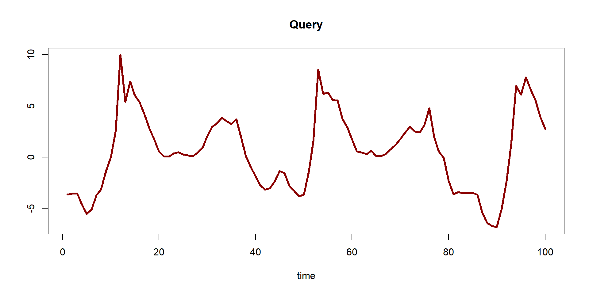
1. Have we ever seen a pattern that looks just like this?

The dataset comes from an accelerometer that records when a person is walking, jogging, or running.

First, let’s load the tsmp library and import our dataset:

# install.packages('tsmp')

library(tsmp)

baseurl <- "https://raw.githubusercontent.com/matrix-profile-foundation/mpf-datasets/a3a3c08a490dd0df29e64cb45dbb355855f4bcb2/"
dataset <- unlist(read.csv(paste0(baseurl, "real/walk-jog-run.txt"), header = FALSE), use.names = FALSE)

And plot it:

plot(dataset, main = "Dataset", type = "l", ylab = "", xlab = "time")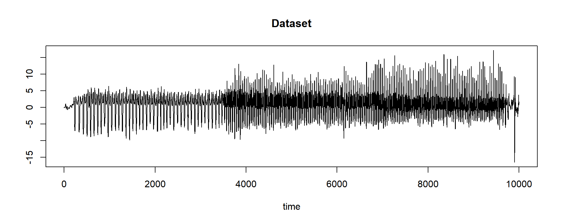

This task is trivial with Mueen’s MASS code…

Here is where tsmp does all for you. All you need is to use the function dist_profile that will return an especial vector called “Distance Profile”. We will talk more about it later in this sequence of posts. This vector is inside the list that is returned by this function:

query <- dataset[5001:5100]  # pretend you didn't see this line. This is the query from the first image above.

# our query has a length of 100 units, we can specify this as `window_size`, but here the
# function will know it.
tictac1 <- Sys.time()
res <- dist_profile(dataset, query)
tictac1 <- Sys.time() - tictac1

cat(paste("dist_profile() finished in ", tictac1, "seconds\n\n"))

## dist_profile() finished in  0.00799798965454102 seconds

str(res)

## List of 3
##  $ distance_profile: num [1:9902] 188 180 174 170 168 ...
##  $ last_product    : num [1:9902] 15.4 21.1 25.7 28.5 29.6 ...
##  $ par             :List of 9
##   ..$ window_size: int 100
##   ..$ data_fft   : cplx [1:16384] 5920+0i -1833-2644i 993-317i ...
##   ..$ data_size  : int 10001
##   ..$ data_mean  : num [1:9902] 0.1029 0.1017 0.101 0.1 0.0994 ...
##   ..$ data_sd    : num [1:9902] 0.4 0.401 0.401 0.401 0.402 ...
##   ..$ query_mean : num 0.602
##   ..$ query_sd   : num 3.73
##   ..$ data       : num [1:10001] 0.01499 -0.04329 -0.00391 -0.03841 0.00122 ...
##   ..$ k          : NULL

What this vector represents is the euclidean distance of our query (the pattern that we want to look for) related to the dataset. This means that the minimum value contains the place that is most similar to our query:

first <- which.min(res$distance_profile)

first  # surprisingly (not) the value is the same as that we used to slice our query...

## [1] 5001

Well, this tells us that at position 5001 there is a pattern that looks like our query. Let’s plot that with a closer look:

plot(dataset, main = "Dataset", type = "l", ylab = "", xlab = "time", xlim = c(4001, 6000))
lines(5001:5100, query, col = 2)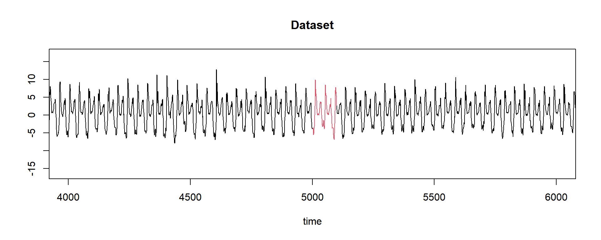

Yes! There is a match! But there are more similar patterns? Here I just find that a new helper function could exist. As it doesn’t, let’s write a few lines (read the comments!):

# This snippet will try to find what we call neighbours, that are patterns that are similar
# to your query, but not the best match.  We know that 'Trivial Matches' happens close to
# the best match, but in this case we are not looking for motifs, but for neighbours. This
# will make sense in the future.

tictac2 <- Sys.time()
st <- sort(res$distance_profile, index.return = TRUE)  # this will order the results and give us the position of them
tictac2 <- Sys.time() - tictac2

cat(paste("sort() finished in ", tictac2, "seconds\n\n"))

## sort() finished in  0.0019989013671875 seconds

# the first one we know already is our best match. Let's now plot the results of three more
# 'matches'.

# Remember that our `window_size` is 100:
w <- 100

plot(dataset, main = "Dataset", type = "l", ylab = "", xlab = "time", xlim = c(4500, 6200))

for (i in 1:5) {
    lines(st$ix[i]:(st$ix[i] + w - 1), dataset[st$ix[i]:(st$ix[i] + w - 1)], col = i + 1, lwd = 2)
    text(st$ix[i], -10, label = paste("match", i), adj = 0, col = i + 1, cex = 0.8)
}

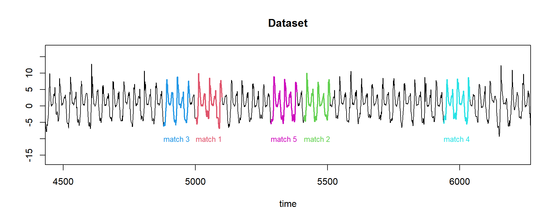
So we did it! We found the five best matches of our query, and it took only 0.00999689102172852 seconds to do it!

This ends our first question of one hundred (let’s hope so!).

Until next time.

next post in this series