100 Time Series Data Mining Questions - Part 2

In the last post we started looking for a known pattern in a time series.

For the next question, we will still be using the datasets available at https://github.com/matrix-profile-foundation/mpf-datasets so you can try this at home.

The original code (MATLAB) and data are here.

Now let’s start:

2. Are there any repeated patterns in my data?

Now we don’t know what we are looking for, but we want to discover something. Not just one pattern, but patterns that repeat, and may look similar or not.

First, let’s load the tsmp library and import our dataset:

# install.packages('tsmp')

library(tsmp)

baseurl <- "https://raw.githubusercontent.com/matrix-profile-foundation/mpf-datasets/a3a3c08a490dd0df29e64cb45dbb355855f4bcb2/"
dataset <- unlist(read.csv(paste0(baseurl, "synthetic/motifs-discords-small.txt"), header = FALSE), 
    use.names = FALSE)

And plot it as before:

plot(dataset, main = "Dataset", type = "l", ylab = "", xlab = "time")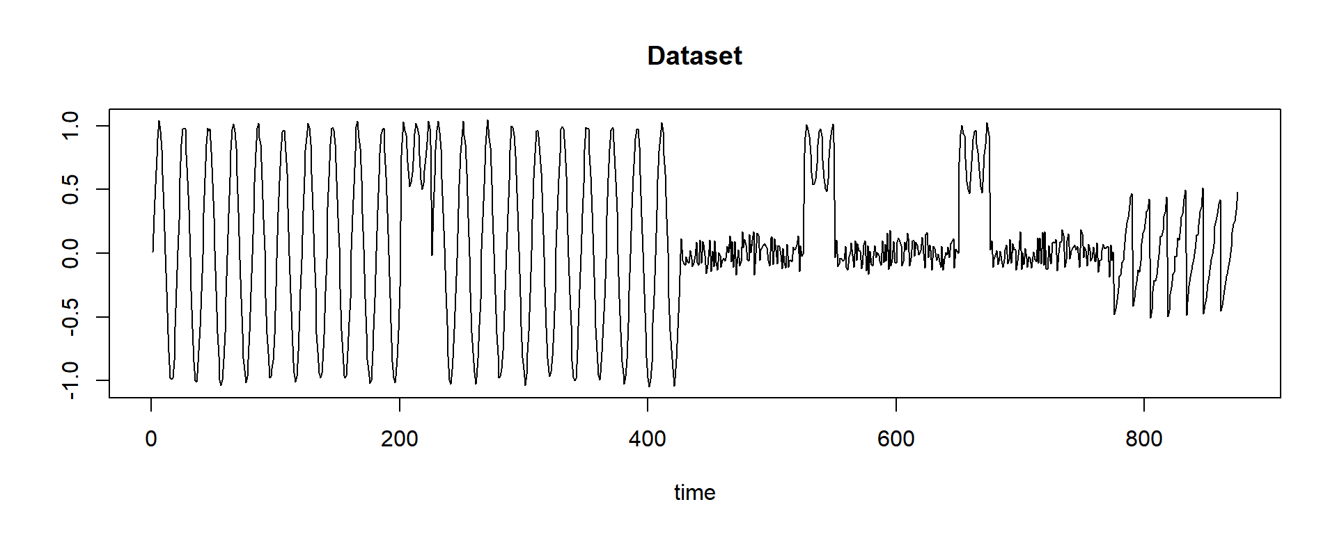

This dataset is a synthetic dataset for demonstration. We clearly see three different patterns. Can we find those patterns?

Again the tsmp does all for you. First I’ll demonstrate how to work with that step by step, and after, using the MPA (Matrix Profile API), introduced by the MPF (Matrix Profile Foundation) has standard functions to use in R and other languages.

In this example, we will not use the Rcpp optimized version of the algorithm, as it is not fully implemented in the package at this moment.

# First, we build our Matrix Profile using the `mpx()` function that is already implemented
# in Rcpp (optimized). We can use other algorithms like STAMP, STOMP, but this is beyond
# the scope of this post.
tictac1 <- Sys.time()
mp_obj <- tsmp(dataset, window_size = 20, exclusion_zone = 1, verbose = 0)
tictac1 <- Sys.time() - tictac1

cat(paste("tsmp() finished in ", tictac1, "seconds\n\n"))

## tsmp() finished in  0.127013921737671 seconds

str(mp_obj, 1)

## List of 9
##  $ mp  : num [1:856, 1] 0.198 0.202 0.203 0.214 0.207 ...
##  $ pi  : num [1:856, 1] 121 122 248 249 250 66 67 48 354 355 ...
##  $ rmp : num [1:856, 1] 0.198 0.202 0.203 0.214 0.207 ...
##  $ rpi : num [1:856, 1] 121 122 248 249 250 66 67 48 354 355 ...
##  $ lmp : num [1:856, 1] Inf Inf Inf Inf Inf ...
##  $ lpi : num [1:856, 1] -Inf -Inf -Inf -Inf -Inf ...
##  $ w   : num 20
##  $ ez  : num 1
##  $ data:List of 1
##  - attr(*, "class")= chr "MatrixProfile"
##  - attr(*, "join")= logi FALSE
##  - attr(*, "origin")=List of 8

Differently of the last post, we don’t have a distance profile but a matrix profile that is the minimum value of all distance profiles of all possible rolling window in this data. Together, we have the profile index that points to the most similar pattern in this data.

Let’s take a look on the matrix profile object:

mp_obj$rmp <- NULL  # we don't need that in this tutorial
mp_obj$lmp <- NULL  # we don't need that in this tutorial
plot(mp_obj, data = TRUE)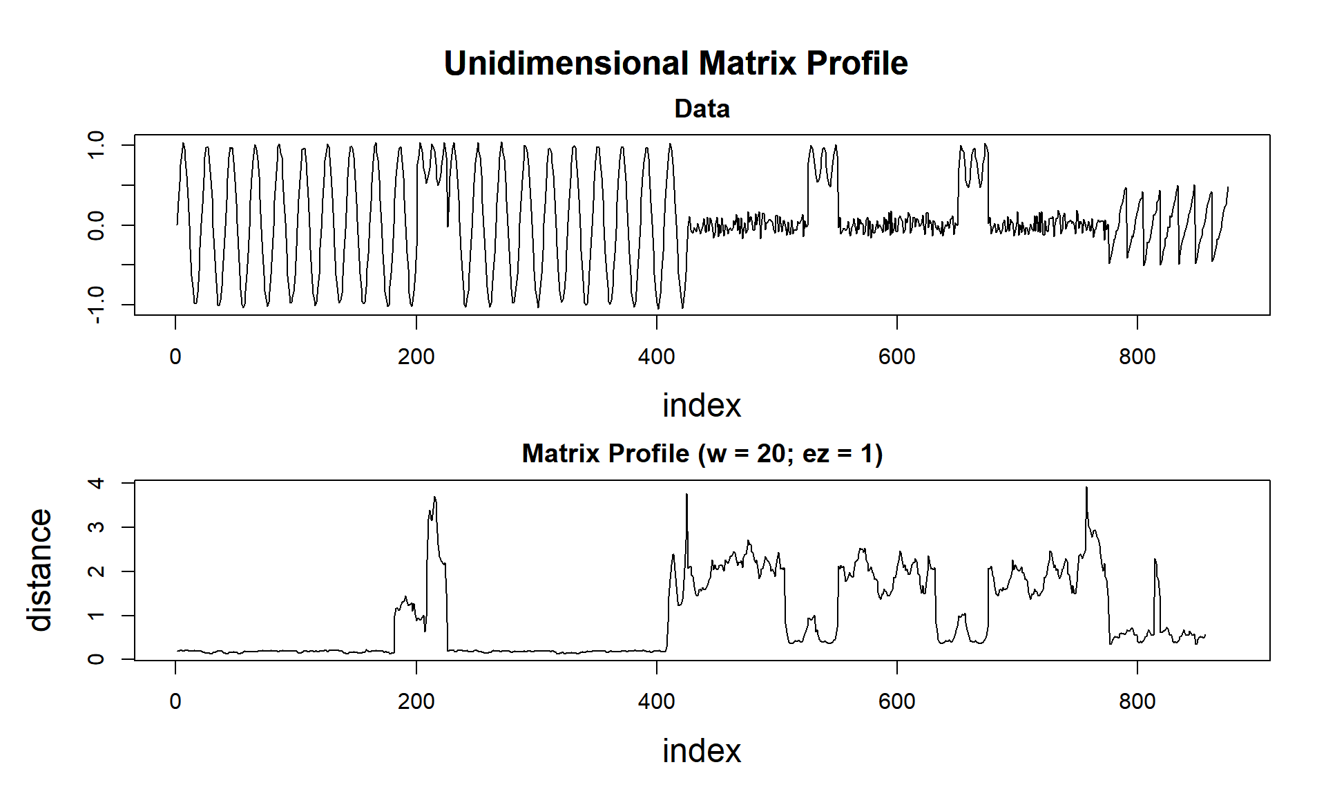

Notice that the Matrix Profile gets lower values as pattern repeats, and higher values when a different pattern arises. Here is the magic!

Continuing trying to find the patterns:

# the `tsmp` package implements the pipe feature from `magrittr` package:
# https://magrittr.tidyverse.org/
tictac2 <- Sys.time()
mp_obj %>%
    find_motif(n_motifs = 3) %T>%
    plot()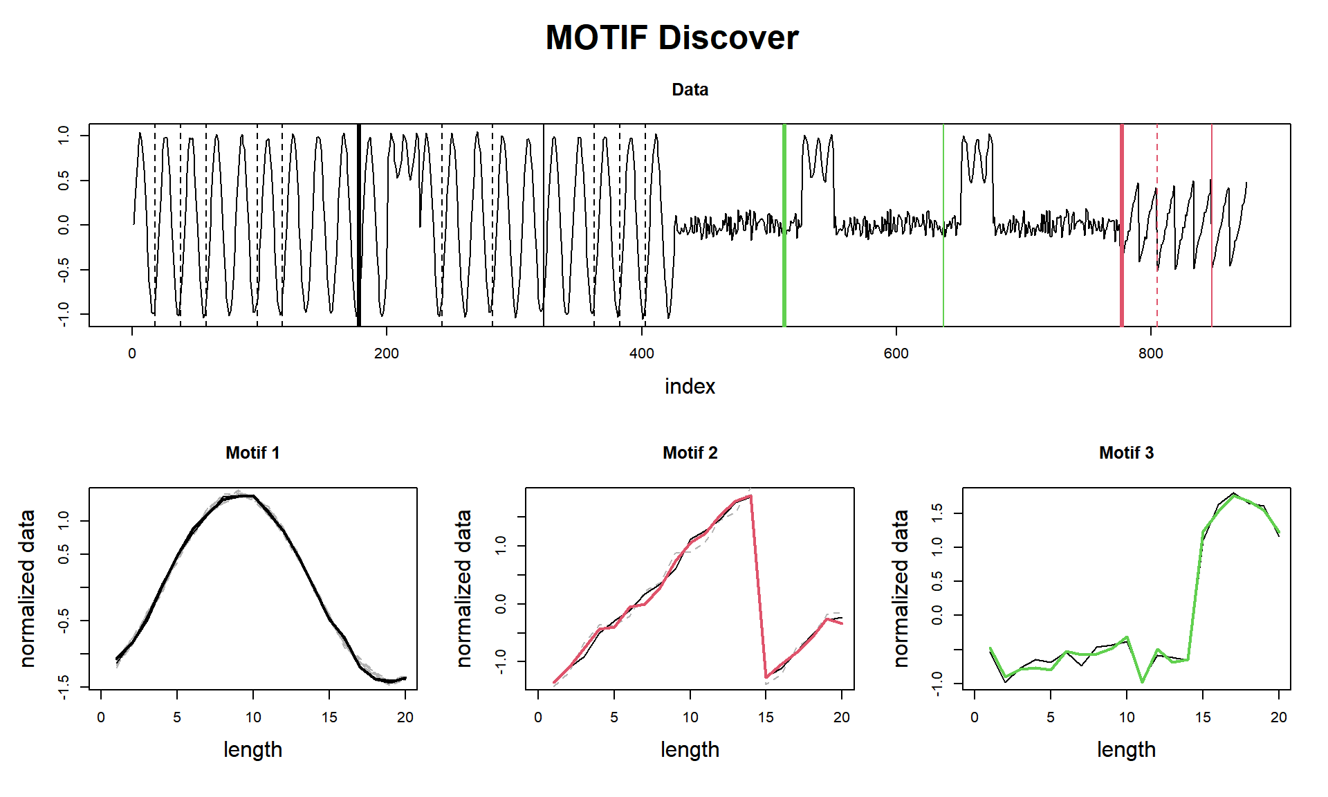

## Matrix Profile
## --------------
## Profile size = 856 
## Window size = 20 
## Exclusion zone = 20 
## Contains 1 set of data with 875 observations and 1 dimension 
## 
## Motif
## -----
## Motif pairs found = 3 
## Motif pairs indexes = [178, 323] [777, 848] [512, 637]  
## Motif pairs neighbors = [363, 283, 58, 383, 98, 38, 18, 118, 403, 243] [805] []

tictac2 <- Sys.time() - tictac2

cat(paste("find_motif() finished in ", tictac2, "seconds (with plot!)\n\n"))

## find_motif() finished in  0.0409982204437256 seconds (with plot!)

Here we see a curious result. I managed to get the three parts, but I confess I did a tweak. As we see, that sinusoidal wave that is in the 3rd motif (the green one) is very similar to the sinusoidal wave from the 1st motif. So why the neighbours (dashed lines) of Motif 1 don’t find that pattern? That’s because of the window_size and exclusion_zone that an eager reader may have seen I set to 1 in tsmp() function, and, I used specifically the window of 20, that fits what I wanted.

I did that on purpose, to seize the opportunity to draw attention to these two parameters. This new concept (Matrix Profile) is almost parameter-free, but these two parameters still essential to know about (later we will see a special feature that can help us to suggest a proper window size).

Anyway, we can see that Motif 3 is a mix of noise and sinusoidal, and that happens two times, so, in essence, this may be considered a motif.

As promised, I’ll use the MPA for a lazy approach:

# You'll see that this approach is way faster, but this is due to programming optimization
# that will be available in later versions.
tictac3 <- Sys.time()
compute(dataset, 64) %>%
    motifs() %>%
    visualize()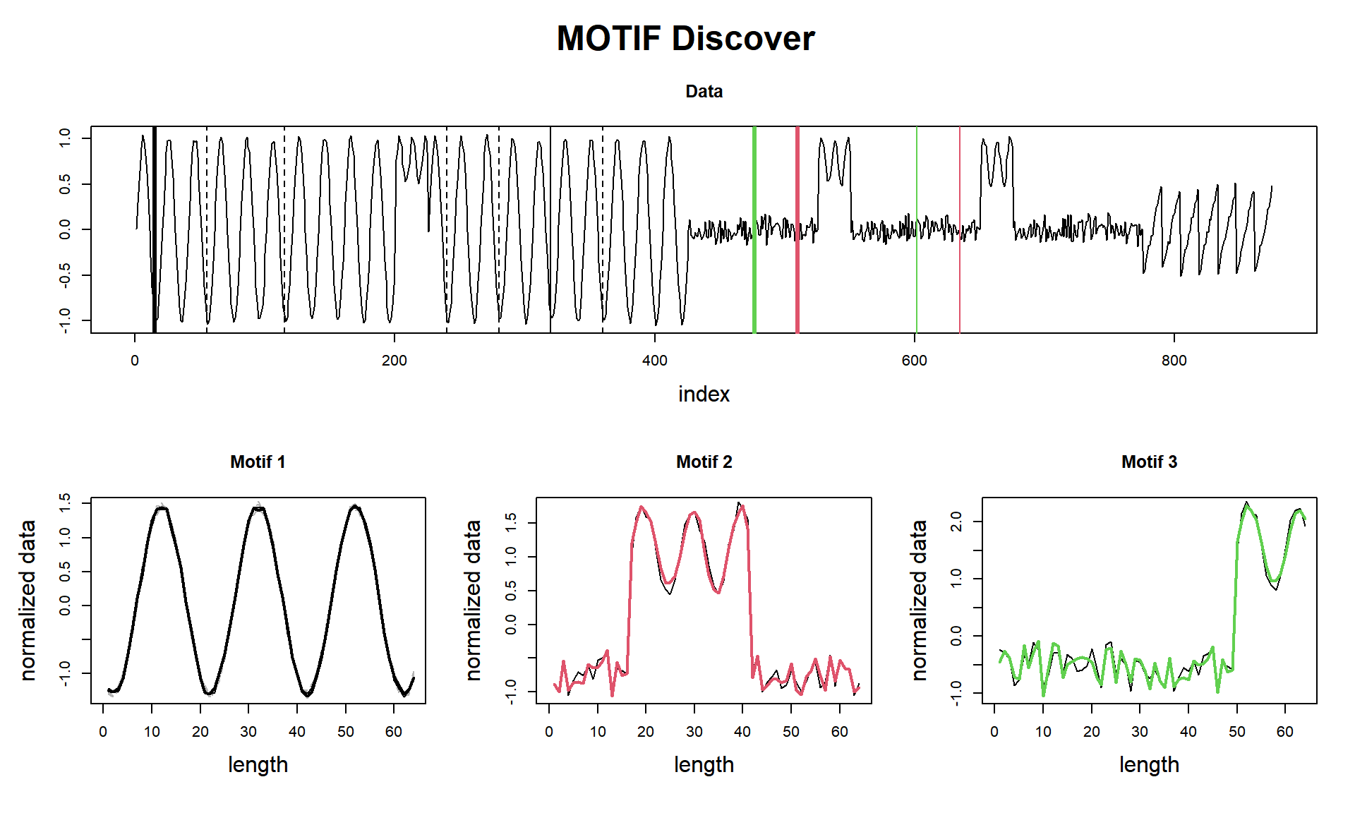

tictac3 <- Sys.time() - tictac3

cat(paste("compute(), motifs(), visualize() finished in ", tictac3, "seconds (with plot!)\n\n"))

## compute(), motifs(), visualize() finished in  0.0807268619537354 seconds (with plot!)

And here is the laziest (spoiler alert! it will plot discords! we’ll talk about them in another post).

# You'll see that this approach is way faster, but this is due to programming optimization
# that will be available in later versions.
tictac4 <- Sys.time()
analyze(dataset, 64)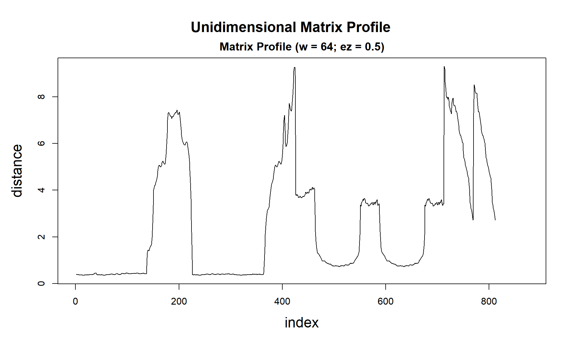

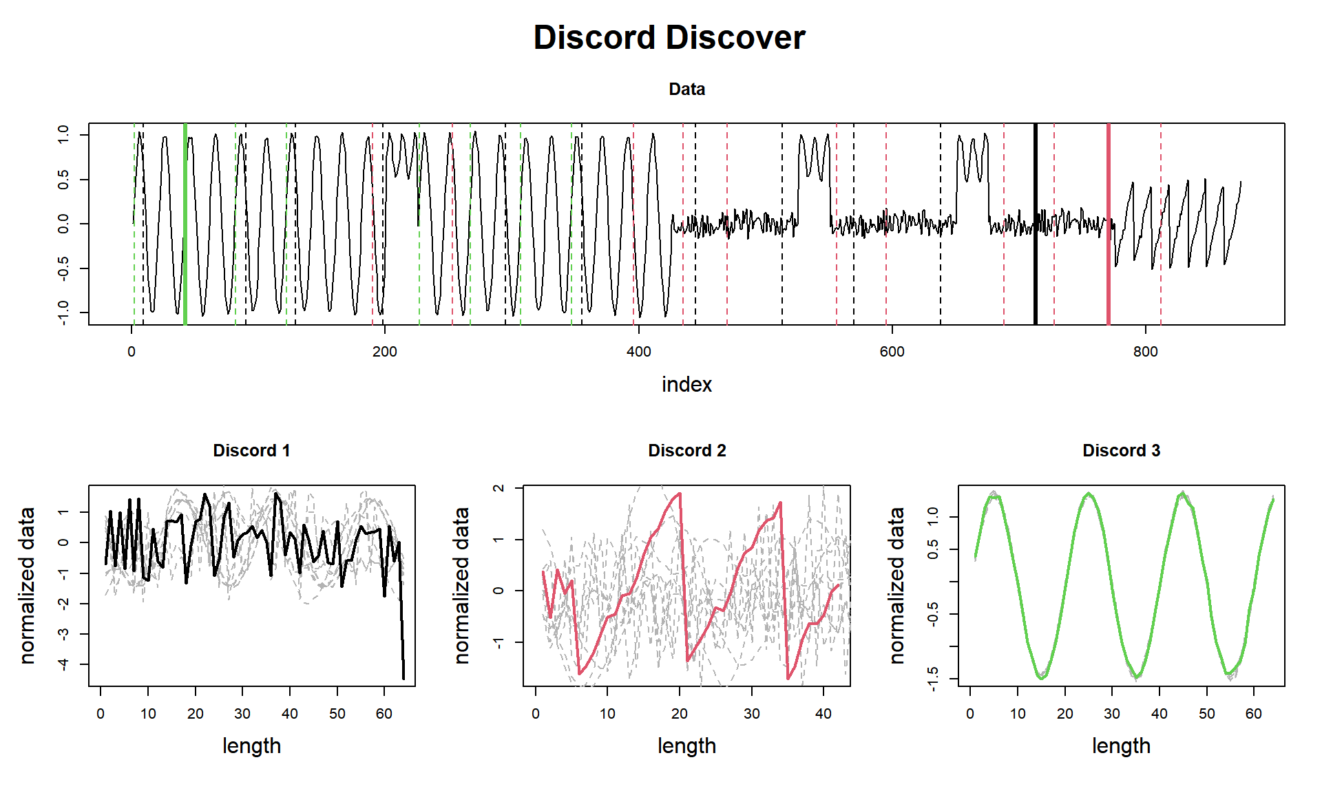
tictac4 <- Sys.time() - tictac4

cat(paste("analyze() finished in ", tictac3, "seconds (with plot!)\n\n"))

## analyze() finished in  0.0807268619537354 seconds (with plot!)

So we did it again!

This ends our second question of one hundred (let’s hope so!).

Until next time.

previous post in this series – next post in this series