100 Time Series Data Mining Questions - Part 6

In the last post took a very long time series, and we summarize it. Now we will do something that seems related when we look at the regime bar: regime change detection.

For the next question, we will still be using the datasets available at https://github.com/matrix-profile-foundation/mpf-datasets so you can try this at home.

The original code (MATLAB) and data are here.

Now let’s start:

6. When does the regime change in this time series?

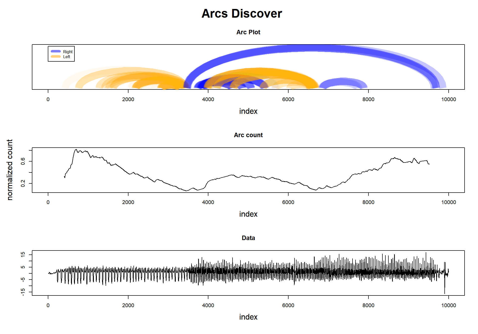
This task exploits another interesting characteristic of Matrix Profile. We know that each position in the Profile Index points to its nearest neighbor. Let’s imagine all these connections as “arcs,” and we will see something interesting: in some regions, it looks like several arcs are pointing to that place. Why’s that?

Imagine, if there is a change in the regime in that time series, we can infer that the nearest neighbor of the previous pattern will not be in the new pattern. It is logical to think that these arcs will tend to be grouped inside each regime region.

Then, how to deal with this feature? Arc counts. Take any point in the time series, and count how many arcs are passing thru that point. The fewer arcs, the greater is the probability that we are changing regimes.

Let’s look to the plot below, where we plot the arcs (not all of them), and in the middle, we see the ‘arc count.’ There we see that there are two valleys, and they match almost precisely where the data changes pattern.

Well, I think I’ve already spoiled all the fun. But, let’s do all the steps anyway:

First, let’s load the tsmp library and import our dataset:

# install.packages('tsmp')

library(tsmp)

baseurl <- "https://raw.githubusercontent.com/matrix-profile-foundation/mpf-datasets/4d99d1bee9b36ca552aa75631748825eda0c064c/"
dataset <- read.csv(paste0(baseurl, "real/PigInternalBleedingDatasetArtPressureFluidFilled_100_7501.txt"), 
    header = FALSE)$V1

And plot it as always:

plot(dataset, lwd = 1, type = "l", main = "Pig Internal Bleeding", ylab = "ABP (mmHg)", xlab = "time")

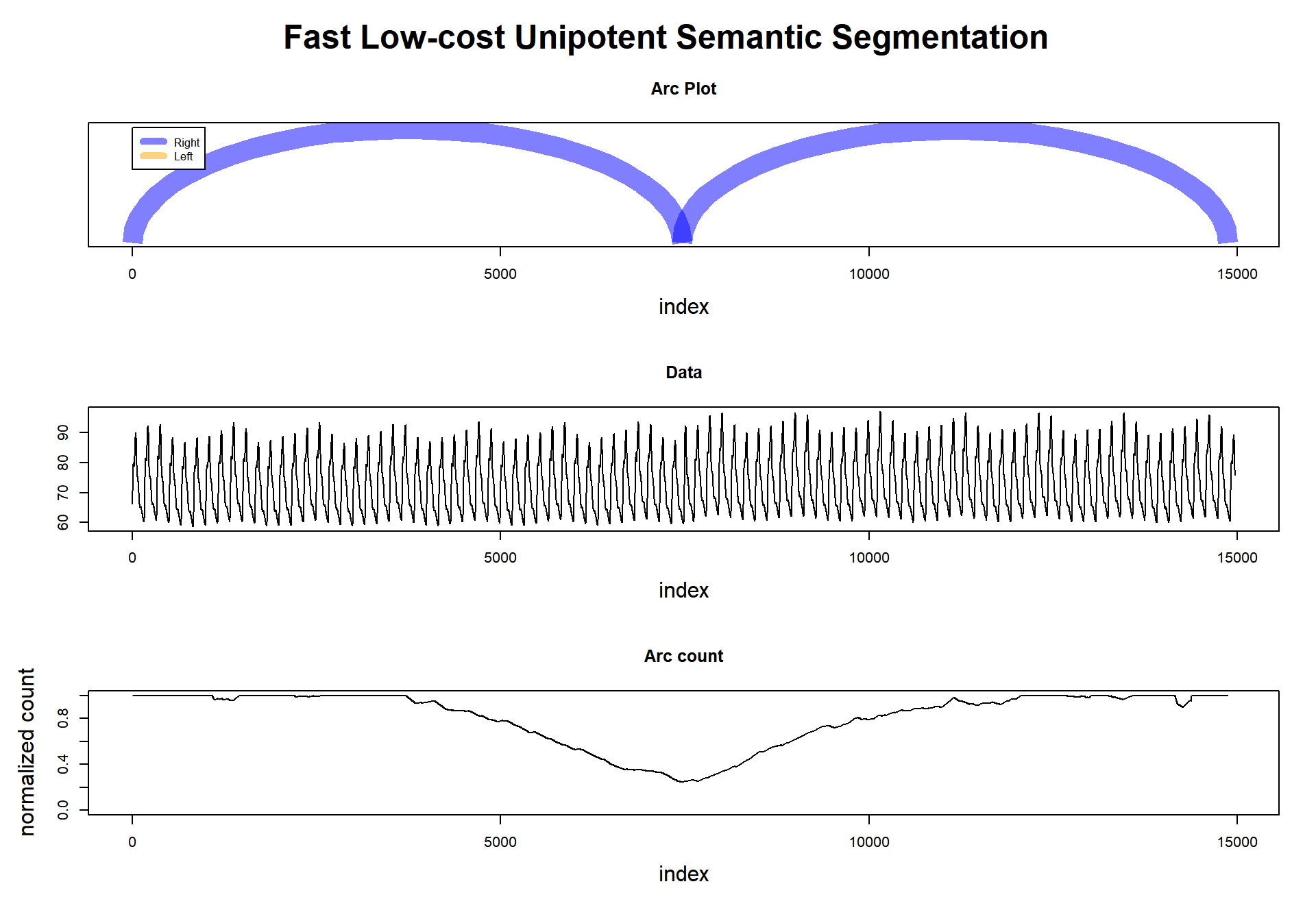
This is not the same dataset from the first figure. This dataset changes only once because it has registered the arterial blood pressure of a pig before and after some bleeding. Well, we can imagine that there will be a regime change. So let’s find it quickly.

Here is the code:

# I'll do this in steps, first compute the matrix profile
mp_obj <- tsmp(dataset, window_size = 100, n_workers = 4, verbose = 0)

# The matrix profile doesn't need to be recomputed, we can apply any mining function on top
# of it, and is fast!
tic <- Sys.time()
mp_obj %>%
    fluss(num_segments = 1) %T>%
    plot

## Matrix Profile
## --------------
## Profile size = 14874 
## Window size = 100 
## Exclusion zone = 50 
## Contains 1 set of data with 14973 observations and 1 dimension 
## 
## Arc Count
## ---------
## Profile size = 14874 
## Minimum normalized count = 0.25 at index 7460 
## 
## Fluss
## -----
## Segments = 1 
## Segmentation indexes = 7460

toc <- Sys.time() - tic
cat("\nFinished in", toc, "seconds\n")

## 
## Finished in 0.1680119 seconds

We can barely see in the dataset where is the regime change, but I tell you that it is at timestamp 7500->7501.

We used a window size of 100 because it is approximately the length of one period of arterial pressure (or the period of whatever repeated patterns you have in your data); however, up to half or twice that value would work just as well. Then the fluss() function managed to extract where was located the minimum arc count, at 7460 (that is incredible near the truth; it is in the middle of the rolling window).

To finalize, see that we set num_segments to 1. This is the only parameter we should care about here. That informs the algorithm of how many changes it needs to look for.

So we did it again!

This ends our sixth question of one hundred (let’s hope so!).

Until next time.

previous post in this series – next post in this series