100 Time Series Data Mining Questions - Part 5

In the last post we managed to find similar patterns between two time series.

For the next question, we will still be using the datasets available at https://github.com/matrix-profile-foundation/mpf-datasets so you can try this at home.

The original code (MATLAB) and data are here.

Now let’s start:

5. If you had to summarize this long time series with just two shorter examples, what would they be?

This is a new kind of question. It’s about summarization, not actually finding motifs.

This task could be addressed using another distance measurement that is more robust than the simple Euclidean distance, but a little bit slower, of course. In fact, this kind of measurement distance can defeat even the DTW based algorithms for this task. It is called MPDist, and the simplest way I can think of explaining it, is: instead of comparing a window of data with the dataset, we compare a shorter rolling window, inside the main rolling window.

This can solve this kind of clustering problem for example:

The dataset is 3 years of Italian power demand data which represents the hourly electrical power demand of a small Italian city for 3 years beginning on Jan 1st 1995 and ending on May 31th 1998. What we want here is to summarize this dataset, showing “Snippets” of data. Snippets are representative patterns present in the data, not rare events like discords, neither (almost) perfectly similar as motifs.

First, let’s load the tsmp library and import our dataset:

# install.packages('tsmp')

library(tsmp)

baseurl <- "https://raw.githubusercontent.com/matrix-profile-foundation/mpf-datasets/05efe885cff4b2266067ad62c4f6fa2b537ad2a2/"
dataset <- read.csv(paste0(baseurl, "real/italianpowerdemand.csv"), header = FALSE)$V1

And plot it as always:

plot(dataset, lwd = 1, type = "l", main = "Italian Power Demand", ylab = "kWh", xlab = "time (hourly)")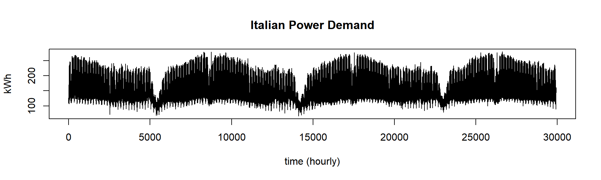

mp_obj <- find_snippet(dataset, 168, 2, 24)
mp_obj %T>%
    plot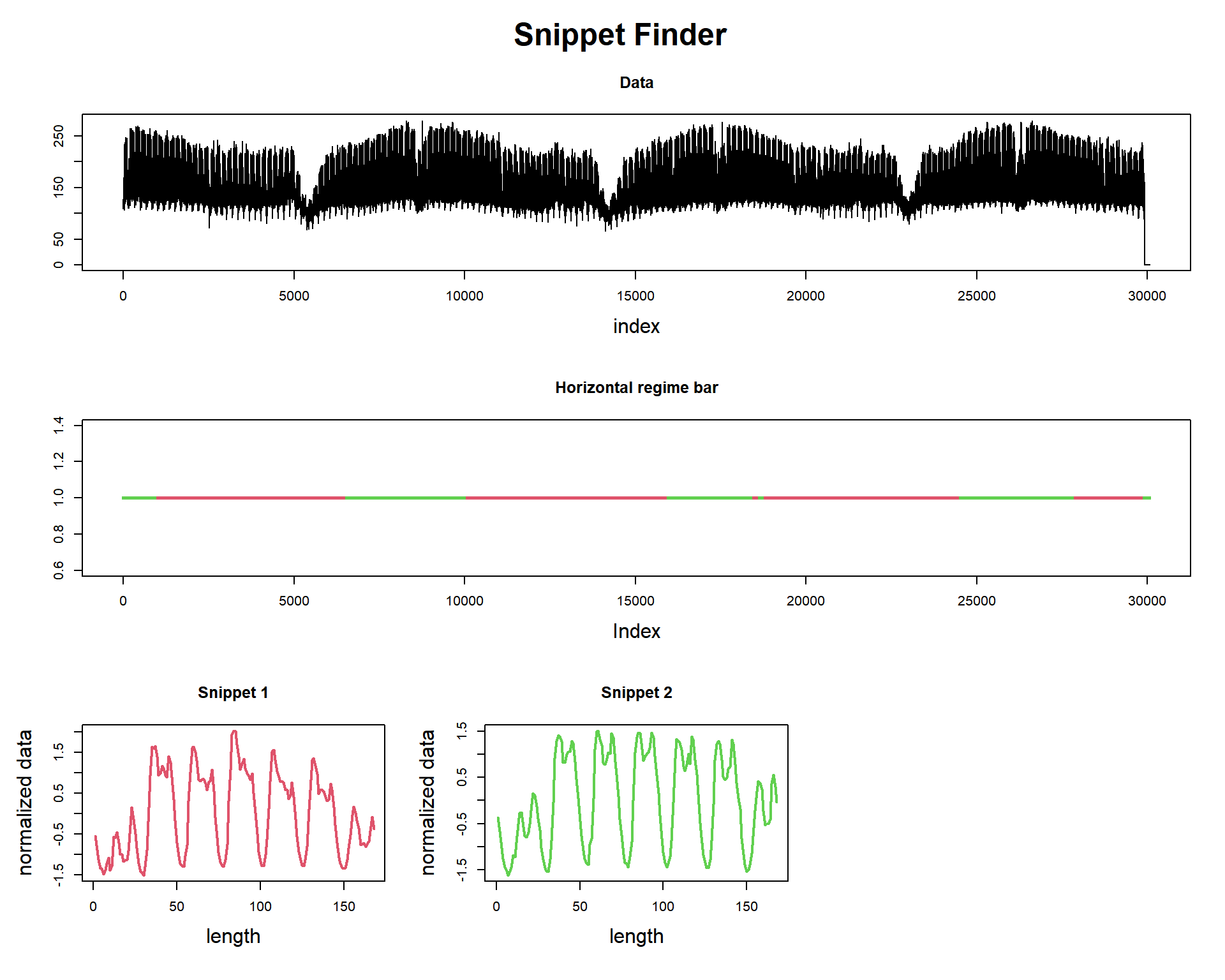

## 
## Snippet
## -------
## Snippets found = 2 
## Snippets indexes = 10921 17977 
## Snippets fractions = 64.25% 35.75% 
## Snippet size = 168

We searched for the top-2 snippets of length 168. This is equivalent to 1 week (7 days). You can see that this way since Jan 1st 1995 is a Sunday, we can confirm that the indexes of each snippet also starts on Sunday (10921 %% 168 is 1 and 17977 %% 168 is also 1). This makes the interpretation easier.

We also obtain the “regime bar,” that tells us which snippet “explains” which region of data. As it happens, These snippets seem to represent summer (red) and winter (green) regimes, respectively. The red line usually stars in later February - early March and ends on October (almost the same period of Daylight Saving Time changes).

Let’s look at the snippets. What makes them different from each other? We see that the “summer” snippet has a lower peak at the end of the day, while the “winter” snippet has a higher peak. This could mean that in the winter, people go home and turn on heaters (for example), and in the summer, people may go home later and doesn’t turn on heaters. This is just a hypothesis, but see that the algorithm gave us the answer: how can I summarize this dataset?

So we did it again!

This ends our fifth question of one hundred (let’s hope so!).

Until next time.

previous post in this series – next post in this series