100 Time Series Data Mining Questions - Part 8

In the last post, we were able to identify when a regime change occurs. Today we will focus on speed (well, a trade-off)

For the next question, we will still be using the datasets available at https://github.com/matrix-profile-foundation/mpf-datasets so you can try this at home.

The original code (MATLAB) and data are here.

Now let’s start:

7. How do I quickly search this long dataset for patterns, if an approximate search is acceptable?

As shown in previous posts, the exact search is surprisingly fast under Euclidean Distance. However, you want more. You don’t have 10 minutes; you need it now! Well, we can do a little trade-off: downsample the data and have an approximate answer. Or, we can use one any-time algorithm (and also have an approximate answer).

I’ll cover both methods here. But first, what is downsample, and what is any-time?

• Downsample may be evident for most readers, but I’ll explain it anyway. Downsample is basically a lower resolution of our data. For example, we can jump every other datapoint and get a new dataset with half of its size (this is the laziest way). We can do better, get the mean of any interval to get a reduced dataset. There are lots of downsampling algorithms available. We will use the PAA algorithm (Piecewise Aggregate Approximation of time series).
• Any-time is an algorithm that can return an answer, well, any-time. This means that the Matrix Profile is being gradually computed and closer to the exact answer, but we stopped earlier and have an approximate result.

We will use the dataset we used for summarization (Italian Power Demand) with about 30k datapoints.

First, let’s load the tsmp library and import our dataset:

# install.packages('tsmp')

library(tsmp)

baseurl <- "https://raw.githubusercontent.com/matrix-profile-foundation/mpf-datasets/05efe885cff4b2266067ad62c4f6fa2b537ad2a2/"
dataset <- read.csv(paste0(baseurl, "real/italianpowerdemand.csv"), header = FALSE)$V1
dataset <- dataset[1:29920]  # here we need to make the data divisible by the value we will use in PAA. This will be fixed in further versions.

And plot it as always:

plot(dataset, lwd = 1, type = "l", main = "Italian Power Demand", ylab = "kWh", xlab = "time (hourly)")

First, we will proceed as usual:

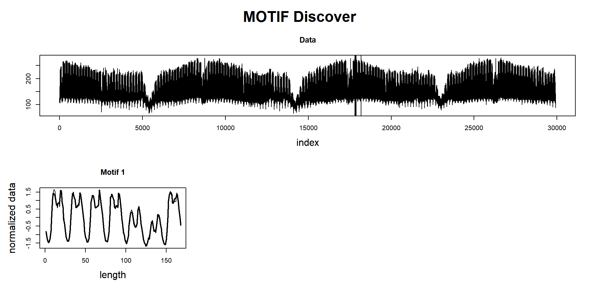
mp_obj <- tsmp(dataset, window_size = 168, n_workers = 4, verbose = 1)

## Warming up parallel with 4 cores.

## Finished in 22.60 secs

Search for motifs:

mp_obj %>%
    find_motif(n_motifs = 1, n_neighbors = 0) %T>%
    plot

## Matrix Profile
## --------------
## Profile size = 29753 
## Window size = 168 
## Exclusion zone = 84 
## Contains 1 set of data with 29920 observations and 1 dimension 
## 
## Motif
## -----
## Motif pairs found = 1 
## Motif pairs indexes = [17859, 18195]  
## Motif pairs neighbors = []

Now, using PAA of 8 (this means the dataset will be 8 times smaller than the original).

mp_obj_paa <- tsmp(dataset, window_size = 168, n_workers = 4, verbose = 1, paa = 8)

## Warming up parallel with 4 cores.

## Finished in 0.91 secs

Search for motifs:

mp_obj_paa %>%
    find_motif(n_motifs = 1, n_neighbors = 0) %T>%
    plot

## Matrix Profile
## --------------
## Profile size = 3720 
## Window size = 21 
## Exclusion zone = 11 
## Contains 1 set of data with 3740 observations and 1 dimension 
## 
## Motif
## -----
## Motif pairs found = 1 
## Motif pairs indexes = [2231, 2273]  
## Motif pairs neighbors = []

A full exact computation takes approximately 20 seconds, and the approximate computation takes less than 1 second and produces (at least in this example) almost exactly the same answer. The answer is just slightly shifted in time. Remember, you need to multiply the indexes by the PAA value.

How well this will work for you depends on the intrinsic dimensionality of your data.

And last but not least, we will use one of the any-time algorithms:

mp_obj_any <- tsmp(dataset, mode = "stamp", s_size = 29920%/%50, window_size = 168, verbose = 1)

## Finished in 2.85 secs

Search for motifs:

mp_obj_any %>%
    find_motif(n_motifs = 1, n_neighbors = 0) %T>%
    plot

## Matrix Profile
## --------------
## Profile size = 29753 
## Window size = 168 
## Exclusion zone = 84 
## Contains 1 set of data with 29920 observations and 1 dimension 
## 
## Motif
## -----
## Motif pairs found = 1 
## Motif pairs indexes = [18543, 27280]  
## Motif pairs neighbors = []

In this example, the any-time algorithm was set to finish after analyzing only 2% of the data, and the answer was incredibly almost the same as the exact computation. Note that it took about 2.5 seconds (slower than using PAA), but here we’ve used the STAMP algorithm that is several times slower than STOMP. And we’ve used only one thread!

So we did it again!

This ends our seventh question of one hundred (let’s hope so!).

Until next time.

previous post in this series