100 Time Series Data Mining Questions - Part 3

In the last post we started looking for repeated patterns in a time series, what we call Motifs.

For the next question, we will still be using the datasets available at https://github.com/matrix-profile-foundation/mpf-datasets so you can try this at home.

The original code (MATLAB) and data are here.

Now let’s start:

3. What are the three most unusual days in this three-month-long dataset?

Now we don’t know what we are looking for, but we want to discover something. Not just one pattern, but patterns that repeat, and may look similar or not.

First, let’s load the tsmp library and import our dataset. In this example, we will use the package xts only because the imported data has a timestamp index and we make more understandable plots, but this is not necessary as we will use basically the values. We will use the window from 2014-10-01 and 2014-12-15 to keep up with the original example from Keogh’s Lab:

# install.packages('tsmp')

library(tsmp)
library(xts)

baseurl <- "https://raw.githubusercontent.com/matrix-profile-foundation/mpf-datasets/a3a3c08a490dd0df29e64cb45dbb355855f4bcb2/"
dataset <- read.csv(paste0(baseurl, "real/nyc-taxi-anomalies.csv"), header = TRUE)
dataset <- xts(dataset$value, as.POSIXct(dataset$timestamp))
tzone(dataset) <- "UTC"
dataset <- window(dataset, start = "2014-10-01", end = "2014-12-15")
events <- xts(c("Columbus Day", "Daylight Saving Time", "Thanksgiving"), as.POSIXct(c("2014-10-13", 
    "2014-11-02", "2014-11-27"), tz = "UTC"))

And plot it as always:

plot(dataset, main = "NYC Taxi anomalies", lwd = 1)

Above we see the taxi load between 2014, October 1st and 2014, December 15th. The data was collected each half-hour. We can see that this data seems to have a well-repeated pattern, but in some days there are some differences. The objective here is to locate what is not normal, or better saying, the discord. Discord is a term that defines the most unusual time series subsequence. Discords have become one of the most effective and competitive methods in anomaly detection.

# We already know the Matrix Profile Object, so I'll skip talking about it.
mp_obj <- tsmp(dataset, window_size = 100, exclusion_zone = 2, verbose = 1)

## Finished in 1.36 secs

## The code below is just to make this easier to explain to the reader.
mp <- mp_obj$mp
attr(mp, "index") <- attr(dataset, "index")
class(mp) <- c("xts", "zoo")
dontplotnow <- plot(mp, main = "Matrix Profile of NYC Taxi anomalies", lwd = 1)
addEventLines(events, srt = -90, pos = 4, on = 0, cex = 0.8, offset = 1.5, col = c(3, 2, 1), 
    lwd = 2)

As we can see above, the Matrix Profile contains three peaks that show us that these areas are very different from the other regions, so they are, as said above, unusual subsequences.

Let’s analyze (ok, I’ve already spoiled the answer in the plot). The most unusual subsequence is located near the Thanksgiving date. (remember, we are using a window size of 100, that means about 2 days, so there is a visible ‘lag’).

The second most unusual subsequence is located around November 6th. And what is that? It is the Daylight Saving Time! The clock going backwards one hour gives an apparent doubling of taxi load.

The third most unusual subsequence is around October 13th, what could it be? Columbus Day! Columbus Day is mostly ignored in much of America, but still a big deal in NY, with its large Italian American community.

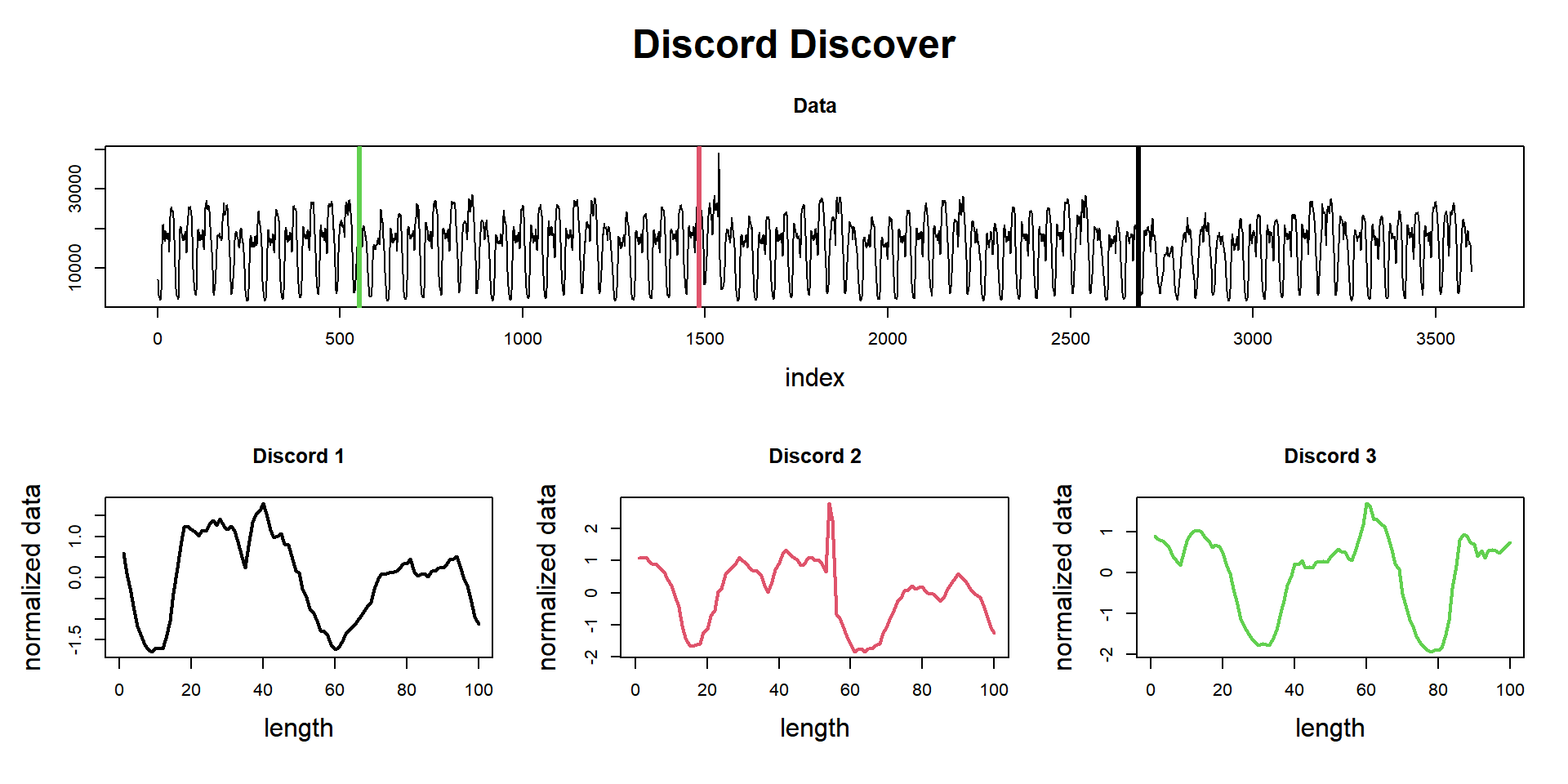
Now let’s use the function find_discord to find these unusual patterns. Notice that I’ve set n_neighbors to zero since I don’t want to look for possible repetition of those patterns, but new, unusual patterns.

# We already know the Matrix Profile Object, so I'll skip talking about it.
mp_obj %>%
    find_discord(n_discords = 3, n_neighbors = 0) %T>%
    plot

## Matrix Profile
## --------------
## Profile size = 3500 
## Window size = 100 
## Exclusion zone = 200 
## Contains 1 set of data with 3599 observations and 1 dimension 
## 
## Discord
## -------
## Discords found = 3 
## Discords indexes = [2686] [1484] [553]  
## Discords neighbors = [] [] []

And here they are. Exactly where we’d foreseen and in the lower part of the potting are the normalized shape of these patterns.

So we did it again!

This ends our third question of one hundred (let’s hope so!).

Until next time.

previous post in this series – next post in this series