100 Time Series Data Mining Questions - Part 4

In the last post we’ve understood and find Discords in our data.

For the next question, we will still be using the datasets available at https://github.com/matrix-profile-foundation/mpf-datasets so you can try this at home.

The original code (MATLAB) and data are here.

Now let’s start:

4. Is there any pattern that is common to these two time series?

Now we will see one of the most interesting and fast jobs that the Matrix Profile can do (there are more, for sure).

In the later tasks, we were comparing a dataset with itself. Now we will compare two datasets, using a rolling window.

This may sound trivial, but as always, you need to know your data.

First, let’s load the tsmp library and import our datasets:

# install.packages('tsmp')

library(tsmp)

baseurl <- "https://raw.githubusercontent.com/matrix-profile-foundation/mpf-datasets/102b8b0451cc9436879c025d21d5709cb4c8a601/"
dataset_queen <- read.csv(paste0(baseurl, "real/mfcc_queen.csv"), header = FALSE)$V1
dataset_vanilla <- read.csv(paste0(baseurl, "real/mfcc_vanilla_ice.csv"), header = FALSE)$V1

And plot it as always:

def_par <- par(no.readonly = TRUE)  # always save the previous configuration
par(mfrow = c(2, 1), cex = 0.8)
plot(dataset_queen, main = "Queen Song", lwd = 1, type = "l", ylab = "", xlim = c(0, 25000))
plot(dataset_vanilla, main = "Vanilla Ice Song", lwd = 1, type = "l", ylab = "", xlim = c(0, 
    25000))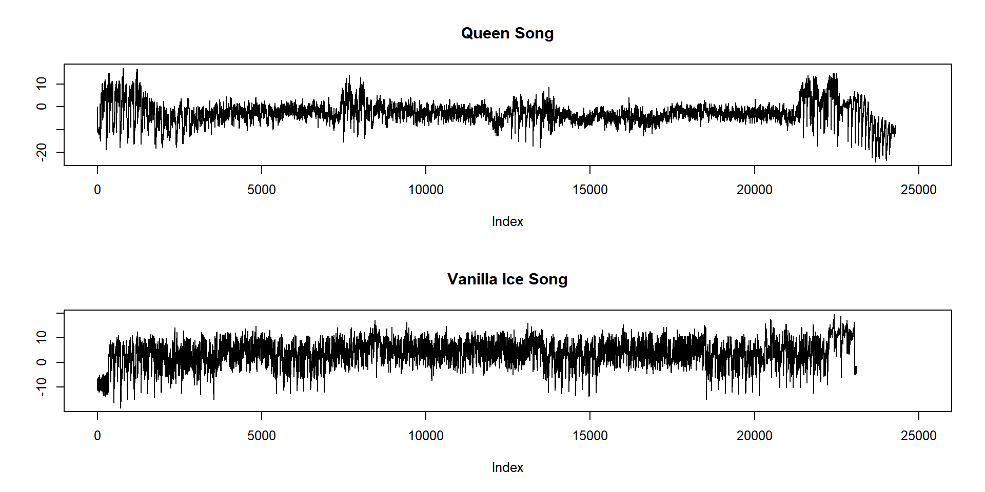

par(def_par)  # and in the end, restore the configurations

Now, remember, know your data. These are sound data. More precisely, these are one of the MFCC representation of these musics that allows us to better represent the sound.

As you may (or not) remember, the MASS algorithm normalizes the data by default, and this may be helpful to find patterns that are basically the same, but differ in amplitude, for example. Here, in this case, normalizing the data would basically mess up with our task! The reason is simple: you can have sequences of the same notes, but with a higher or lower pitch, so they are not the same.

In this case, we will use the SiMPle algorithm that uses a non-normalized version of MASS.

# First we will crop the Queen to be the same size of Vanilla Ice
dataset_queen <- dataset_queen[1:length(dataset_vanilla)]
# and use the SiMPle algorithm. This algorithm is not optimized yet... so it takes more
# time.
mp_obj <- simple_fast(cbind(dataset_queen, dataset_vanilla), window_size = 300, exclusion_zone = 1, 
    verbose = 1)

## Finished in 27.44 secs

# and now let's plot all together:
def_par <- par(no.readonly = TRUE)  # always save the previous configuration
par(mfrow = c(3, 1), cex = 0.8)
plot(dataset_queen, main = "Queen Song", lwd = 1, type = "l", ylab = "", xlim = c(0, 25000))
plot(dataset_vanilla, main = "Vanilla Ice Song", lwd = 1, type = "l", ylab = "", xlim = c(0, 
    25000))
plot(mp_obj$mp, main = "Matrix Profile", lwd = 1, type = "l", ylab = "", xlim = c(0, 25000))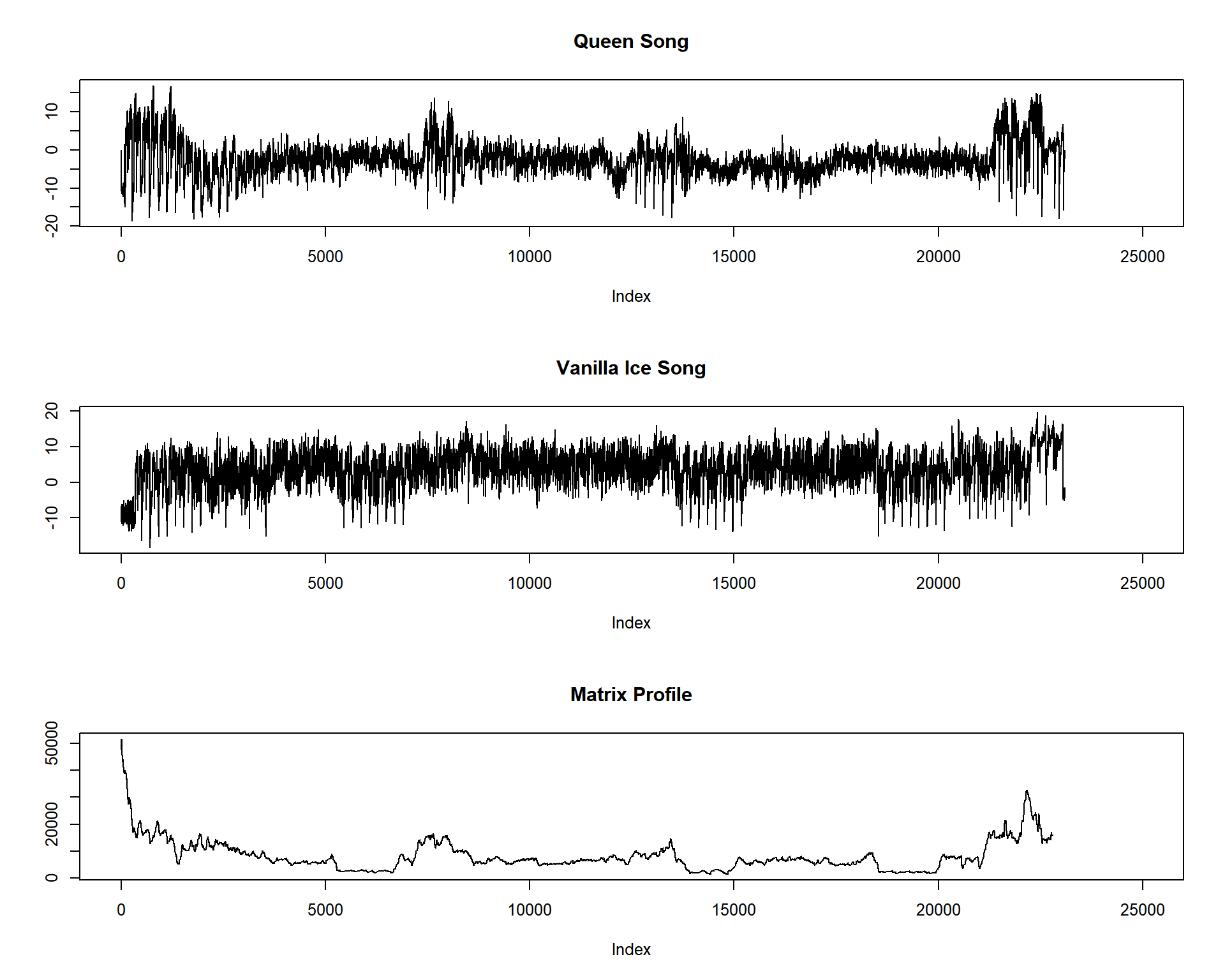

par(def_par)  # and in the end, restore the configurations

You can see that the lower parts of the Matrix Profile align well with that famous bassline from “Under Pressure” by Queen which was plagiarized by Vanilla Ice.

So we did it again!

This ends our fourth question of one hundred (let’s hope so!).

Until next time.

PS: When I was writing this post, I realized that the tsmp package lacks some tools to better visualize what is going on with the SiMPle approach. I promise that in a later version of the package I’ll cover this issue, and get back to this post.

previous post in this series – next post in this series